For data teams, the clock is always ticking. In a business landscape defined by rapidly expanding datasets, slow queries can grind insights to a halt. That's why performance tuning is especially critical when working with a platform like Snowflake. This platform, renowned for its lack of traditional indexes, presents unique challenges and opportunities for optimizing query performance. To navigate these uncharted waters, data engineers and analysts need a mastery of specialized optimization tactics. Join me as we dive into the art of writing fast code that unlocks the full capabilities Snowflake offers. We’ll review examples ranging from basic query tuning to more advanced optimizations that can mean the difference between swift analytics and stalled projects.

Snowflake Performance Tuning Strategy

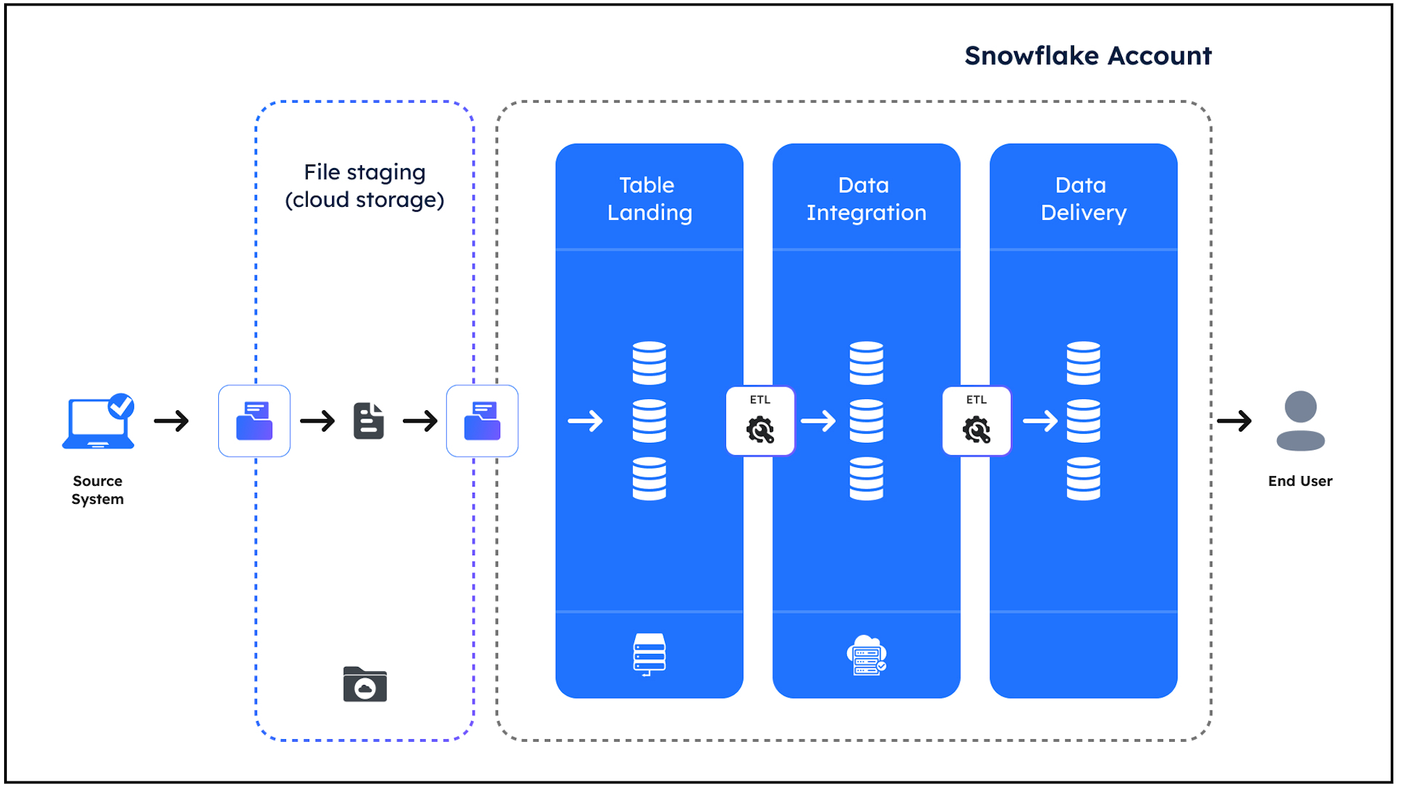
Before we start, let’s put the overall performance-tuning strategy in context. The diagram below illustrates the typical data processing pipeline you’ll see on any Snowflake platform, which consists of the following:

• Data Loading: This involves copying data from Cloud Storage into a Table Landing zone. This normally uses the Snowflake COPY or SNOWPIPE commands.

• Data Transformation: Data from multiple sources and loading into Data Integration and Data Delivery zones. This involves the execution of Insert, Update, or Merge statements to clean, manipulate, and transform the data ready for consumption.

• Data Querying & Consumption: The data by end user dashboards, reports, or analysis. This typically involves SELECT statements against the Data Delivery zone.

It’s worth considering the above because the approach and solutions tend to differ. Let’s consider each in turn.

Data Delivery

As indicated above, data delivery is all about quickly using SELECT statements to deliver results to end-users. This means it's vital SQL is tuned for maximum performance. When tuning query performance, the first place to look is the query profile.

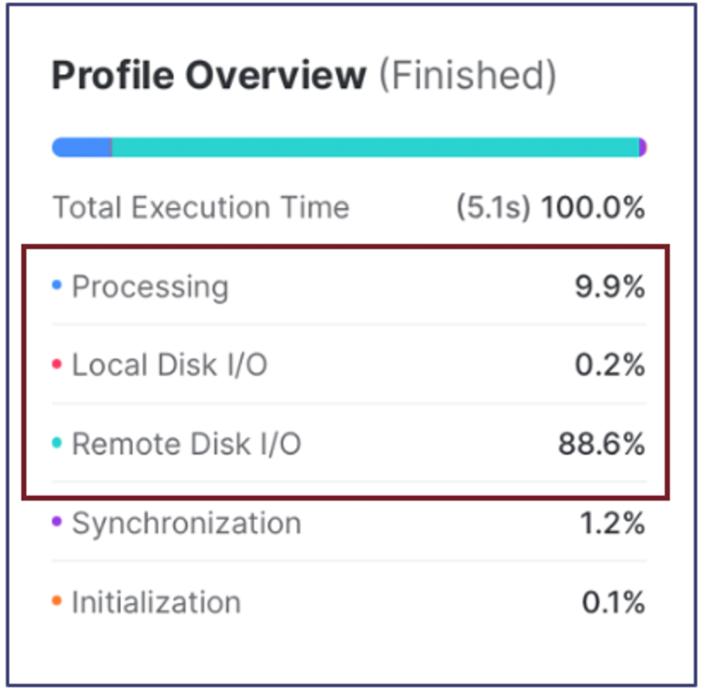
The screenshot above illustrates the first place to check for performance issues. Many assume this indicates the time spent, but it's the time waiting for resources.

The above case shows the query spent just 10% of its time waiting on CPU resources, almost zero (0.2%) of the time waiting for Local Disk I/O to complete, but nearly 90% of the time waiting on Remote Disk I/O.

Reviewing the overall Snowflake hardware architecture illustrated in the diagram below is helpful to understand what this means.

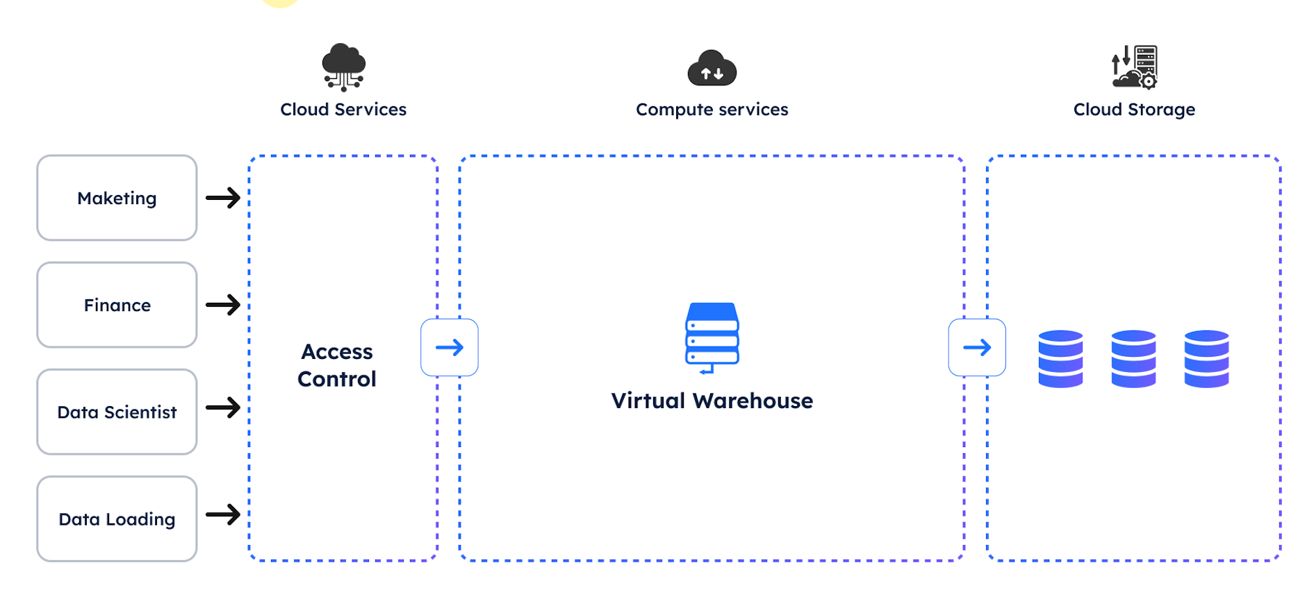
The above diagram shows how queries submitted to Snowflake are handled by the Cloud Services Layer, determining the best way to execute the query. The SQL is then passed to a Virtual Warehouse, a physical computer with CPU cores, memory, and SSD (Local) storage.

When queries are executed, the data is read from Remote Storage, cached in SSD, and results computed and returned to the user.

The key insight here is that (SSD) Local Storage is hundreds of times faster than Remote (disk) storage. One of the most effective ways to maximize query performance is limiting Remote Disk accesses.

The most effective way to reduce remote disk I/O is using the query WHERE clause to filter out rows. Complex SQL queries often include a series of Common Table Expressions (CTEs or inline views), and the best practice is to filter out rows as early as possible. The fewer rows fetched from the Remote Disk, the faster the query executes.

The next step in tuning Snowflake query performance is to review the query statistics illustrated in the screenshot below.

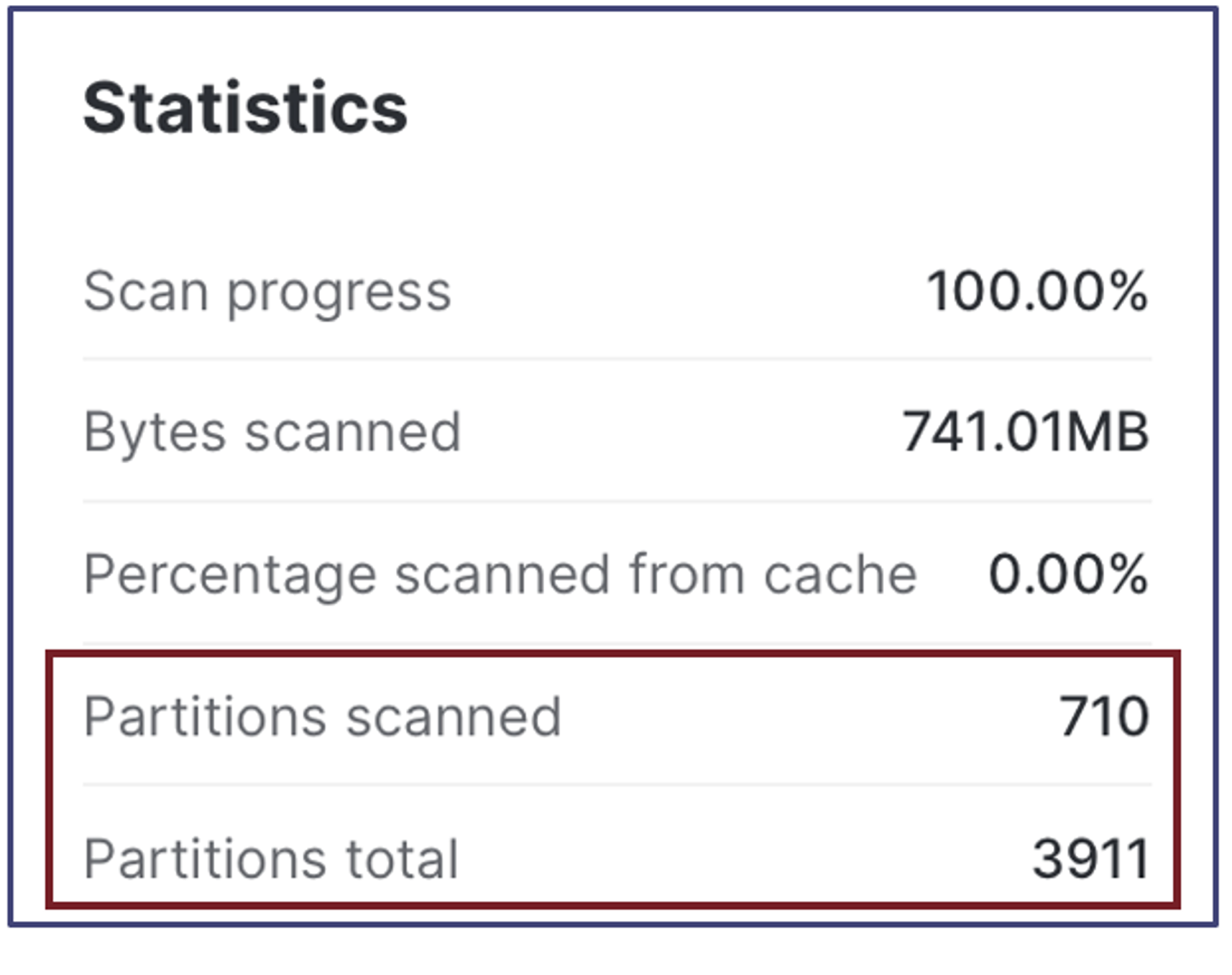
Snowflake stores data in 16MB blocks called micro partitions and automatically prunes these to maximize query performance, but it's entirely dependent upon the WHERE clause. If (for example), a query includes no WHERE clause, Snowflake will need to fetch the entire table from Local or Remote storage with a significant impact upon performance.

Tuning the query WHERE clause

You can make simple changes to the WHERE clause to maximize query performance. Take, for example, the following SQL statement:

select *
from SNOWFLAKE_SAMPLE_DATA.TPCH_SF1000.ORDERS
where to_char(o_orderdate,'DD-MON-YYYY') = '01-APR-1992';

The above query returns ORDERS placed on 1st April 1992. However, we limited Snowflake's ability to prune query performance automatically because we formatted the O_ORDERDATE as a character in the WHERE clause.

select *
from SNOWFLAKE_SAMPLE_DATA.TPCH_SF1000.ORDERS
where o_orderdate = to_date('01-APR-1992','DD-MON-YYYY');

The above query produces the same result ten times faster, completing in under four seconds instead of nearly 40 seconds. The reason is we left the O_ORDERDATE column unmodified.

Surprisingly, despite converting a DATE to a CHARACTER field, Snowflake can still perform some partition pruning. However, modifying WHERE clause columns using a user-defined function will almost certainly lead to a full table scan.

select *
from orders
where format_date_udf(o_orderdate,'DD-MON-YYYY') = '01-APR-1992';

The above query will perform even worse as Snowflake cannot evaluate the output of a User-Defined Function and will always lead to a full table scan.

Tuning Sort Operations

Designing an analytics solution without including an ORDER BY or GROUP BY clause in the query is almost impossible. However, sorts are the most computationally expensive operations and are often the most significant cause of query performance issues.

Often, data analysts need to determine whether a given column is unique and will execute the following SQL:

select count(distinct l_orderkey)
from snowflake_sample_data.tpch_sf1000.lineitem;

However, the following query will execute around 600% faster with an accuracy of around 99%:

select count_approx_distinct(l_orderkey)
from snowflake_sample_data.tpch_sf1000.lineitem;

The COUNT_APPROX_DISTINCT is one of a series of approximation functions that accurately estimate large data volumes orders of magnitude faster.

Dealing with high-cardinality data

While dealing with large data volumes is often necessary, you should be especially careful when sorting high cardinality data, for example, by a unique key. Take, for example, the following SQL statements, which appear similar but have wildly different query performance.

Query 1 - Unique Key

select o_orderkey,
       sum(o_totalprice)
from orders
group by 1;

Query 2 - Low Cardinality

select o_orderpriority,
       sum(o_totalprice)
from orders
group by 1;

You may be surprised to find that query 2 (Low Cardinality) runs around 22 times faster than query 1 (Unique Key), as illustrated in the screenshot below:

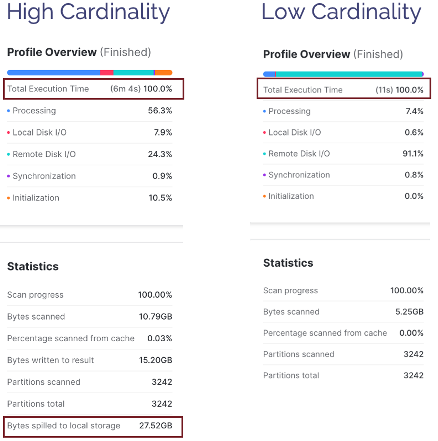
The reason for the huge query performance difference is that Query 1 - Unique Key (which takes over six minutes to complete), includes a GROUP BY on a column with 1.5 billion unique values whereas Query 2 - Low Cardinality (executing in 11 seconds) has just five distinct values.

In this case, the best practice is to be aware of the high cost of sort operations and avoid GROUP BY or ORDER BY operations on highly unique keys.

Using the Snowflake LIMIT or TOP option

There are sometimes use cases where we need to ORDER very large data volumes by unique keys, but it’s still possible to improve query performance using the simple LIMIT or TOP options on SELECT statements.

Consider the following SQL statements:

Query 1 - Order by Every Row

select *
from lineitem
order by l_quantity;

Query 2 - Order by With Limit

select *
from lineitem
order by l_quantity
limit 10;

Using the LIMIT 10 option on Query 2 (only first ten rows), leads to an 11 times improvement in query performance from over 17 minutes to just 1m 35s.

The reason for the huge difference in query performance is revealed in the Query Plan. Query 1 (Order by every row) on the left includes a Sort operation that returns 600 million rows, whereas Query 2 (order by with limit) on the right uses a SortWithLimit operation to reduce the entries from 600m to just 10.

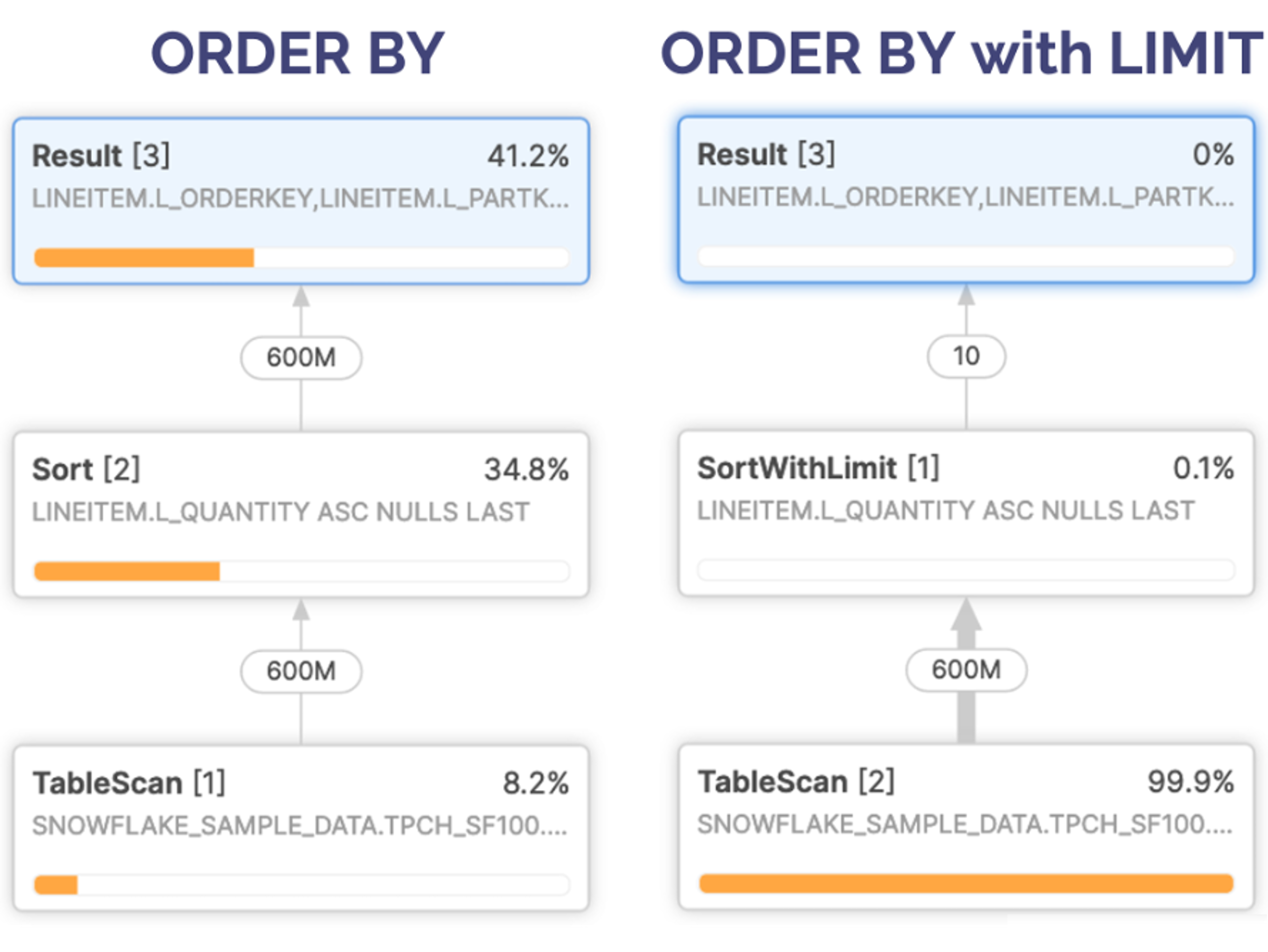
Another significant contributor to the query performance is that the Order by with limit scans half the number of micro-partitions and eliminates spilling to storage, significantly reducing query execution time.

Spilling to Storage

The diagram below illustrates the internal structure of an XSMALL virtual warehouse. It (currently) consists of eight CPU cores, gigabytes of memory, and hundreds of gigabytes of fast SSD storage attached to slower Remote Storage.

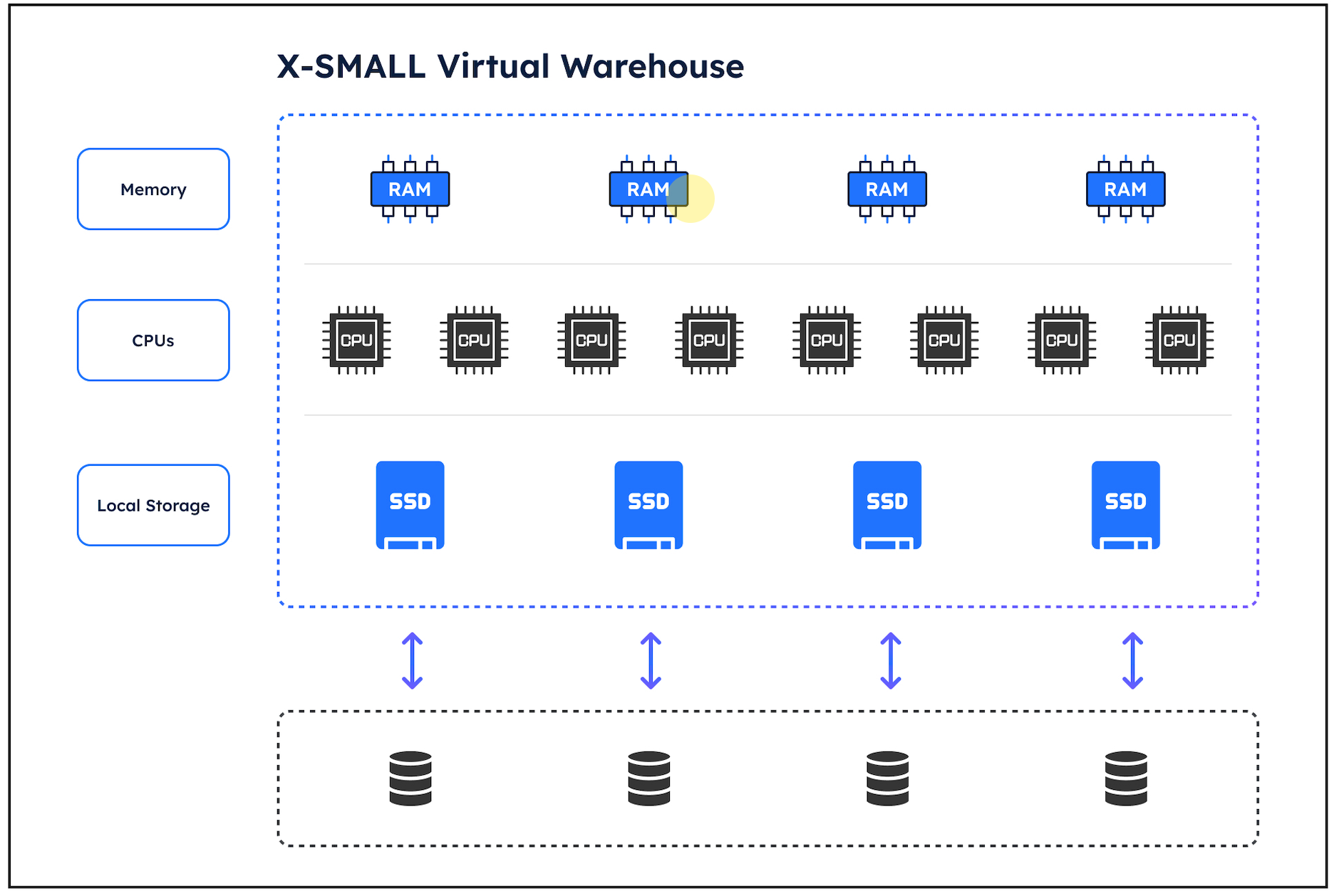
When Snowflake executes a query with an ORDER BY or GROUP BY clause, it must sort the results it attempts to complete in super-fast main memory. However, sorting large data volumes in a smaller warehouse runs out of memory and needs to spill working data to SSD, which is thousands of times slower.

When sorting even bigger data volumes, it may need to spill to Remote Storage, which is many hundreds of times slower again.

It’s good practice to avoid spilling to storage where possible, but how to do this?

There are several Snowflake best practice tuning strategies to avoid spilling to storage, including:

1. Reduce sort volume: Similar to the best practices above, this involves using the WHERE clause to filter out results as early as possible to reduce the number of sorted rows.

2. Use a LIMIT: As we can see above, a LIMIT clause is pushed down into the query, eliminating spilling to storage with a huge improvement in Snowflake query performance.

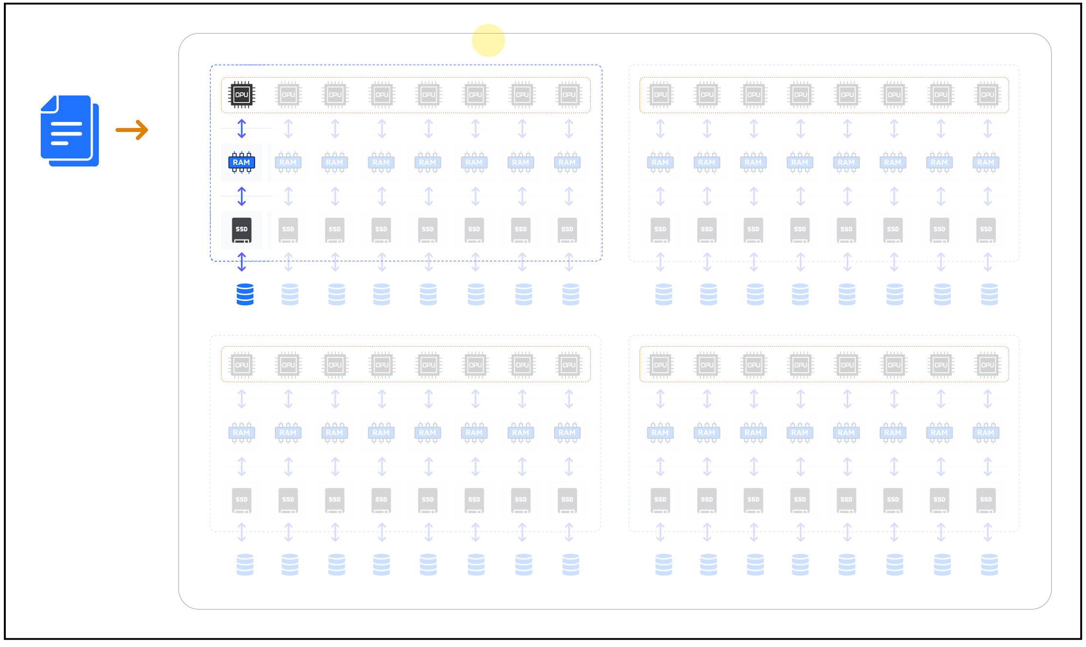
3. Scale Up: The diagram below illustrates the internal structure of a MEDIUM-size warehouse, which includes four servers**.** By scaling up to a larger warehouse, we can spread the workload across multiple servers, which gives (in this case) four times the memory and SSD, which is the simplest way to resolve the issue.

4. Cluster the Data: A final (although sometimes challenging) approach involves clustering the data by the sort key. This often eliminates the SORT operation and can have a massive impact on query performance.

Clustering the Data

The quickest and most simple way of clustering data is to sort it by one or more columns. The SQL snippet below will produce a sorted version of a table:

insert overwrite into orders
select *
from orders
order by o_orderdate;

The above query replaces the contents of the ORDERS table with data sorted by ORDER DATE, which means any GROUP BY or ORDER BY won’t need to sort the data. This approach is, however, not without its drawbacks, and it’s worth reading the article Snowflake Clustering Keys Best Practice for further guidance.

Maximizing Snowflake Data Transformation Performance

Data Transformation involves fetching, cleaning, merging, and transforming data into a form suitable for end-user consumption, and this often accounts for 60-80% of the overall system cost. It, therefore, must be the primary focus for Snowflake query tuning. In addition to producing results faster, tuning transformation jobs can significantly impact Snowflake's cost.

Avoid row-by-row-processing

Data Engineers and Data Scientists have the option to execute procedural code against Snowflake using Python, Java, Javascript and Snowflake Scripting in addition to Scala using Snowpark. There's a risk however, that coding in a language which supports LOOPS, leads to repeated single-row query execution - also know as "Row-by-Row" processing.

Row by Row Processing - is "Slow-by-Slow" - Tom Kyte

One of the most important query-tuning best practices on Snowflake is to avoid row-by-row processing. Unlike on-premises databases like Oracle, Snowflake is designed primarily for set-at-a-time processing of large data volumes rather than single-row inserts, updates, or deletes.

Take the following row-by-row solution, which takes around ten seconds to copy just ten rows into the CUSTOMER table:

declare
v_counter number;
begin
  for v_counter in 1 to 10, do
     insert into customer
     select *
     from snowflake_sample_data.tpcds_sf100tcl.customer
     limit 1;
  end for;
end;

Then, consider the following set-at-a-time query that copies data from the same table in 9.4 seconds on an XSMALL warehouse.

insert into customer
select *
from snowflake_sample_data.tpcds_sf100tcl.customer
limit 15000000;

In conclusion, using set-at-a-time queries, Snowflake can process fifteen million rows simultaneously as row-by-row processing copies ten rows. That’s a performance improvement of 1.5 million times.

The only exception to the above scenario is when dealing with Snowflake Hybrid Tables, designed for OLTP-type applications processing single-row DML operations in milliseconds.

Scale up for larger Data Volume.

This best practice is true for almost any end-user or transformation queries and involves executing long-running queries on a larger virtual warehouse.

In principle, provided the query workload can be distributed across all the available servers, any query will run twice as fast on the next warehouse size. Consider the following table showing the benchmark results of copying a 1.3 TB table on different warehouse sizes.

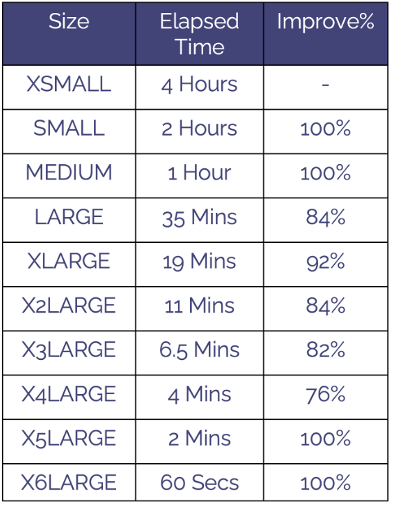
The results above demonstrate very large data volumes can be scaled from an XSMALL warehouse running for four hours to an X6LARGE in just 60 seconds. Notice the improvement is around 76% to 100% each time. This is the most important key performance indicator (KPI) when warehouse sizing. Provided the workload completes around twice as fast each time, it’s worth trying the workload on the next size up.

The challenge of identifying the optimum warehouse size is illustrated in the diagram below.

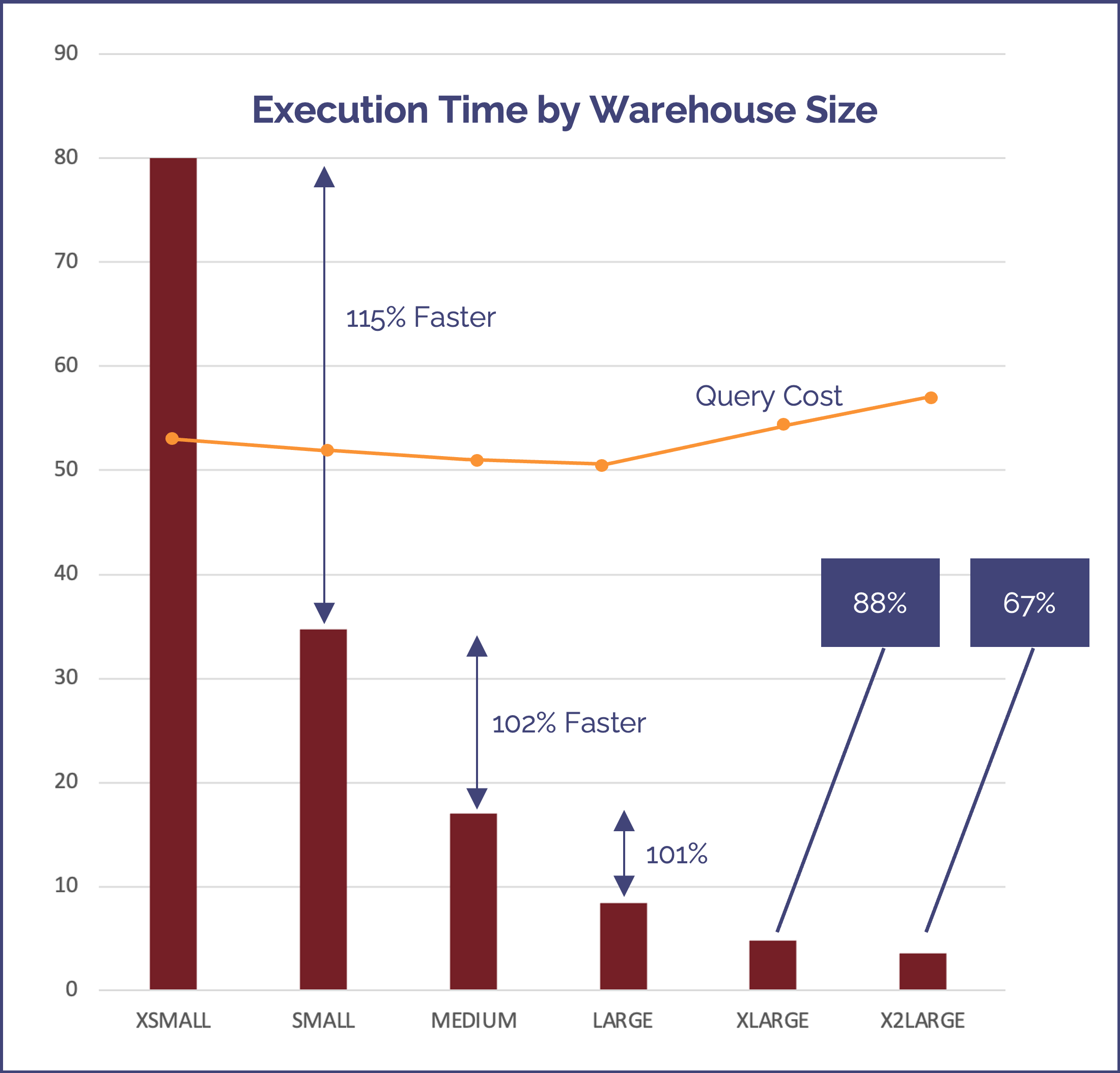
The above diagram shows the performance of a benchmark query executed on an XSMALL to X2LARGE warehouse. In this case, the query processed a relatively small data volume (several gigabytes), and although each time we scaled up to a larger warehouse, (for example from an XSMALL to a SMALL), the query was executed twice as fast.

Since the charge rate per second doubles with warehouse size, we can conclude that each step where the performance is at least double, that the cost will remain the same.

Snowflake has an amazing super-power. You can often get the same work done twice as fast for the same cost. - Kent Graziano (The Data Warrior)

However, each time the performance gain is less than 100%, it costs slightly more, although of course you get the extra performance improvement.

For example, running the query on an XLARGE warehouse would cost 12% more than a LARGE warehouse for an 88% performance improvement.

The real insight here, however, is that the query time is reduced from 80 minutes on an XSMALL warehouse to just 8 minutes on a LARGE for the same cost.

Be aware though, there's almost no performance benefit in scaling up relatively simple, short running queries. The best approach is to execute your workload (all the queries for a given job or set of dashboard users), on a warehouse size, and then scale up until the performance improvement is less than 100%.

Maximizing Snowflake Data Loading Performance

One of the single biggest mistakes made by data engineers is assuming a COPY operation will execute faster on a bigger virtual warehouse. The correct answer is, yes, it will, but it depends.

If you execute the following SQL to load data files from the @SALES stage, Snowflake will use the currently assigned virtual warehouse to load data into the SALES table. Let’s assume you use a MEDIUM-size warehouse to maximize load performance.

copy into sales
from @sales_stage;

If you’ve only a single file to load, the diagram below illustrates how Snowflake executes the COPY operation using a single CPU.

In summary, this won’t improve COPY performance and will take the same time to load on a MEDIUM-size warehouse as an XSMALL.

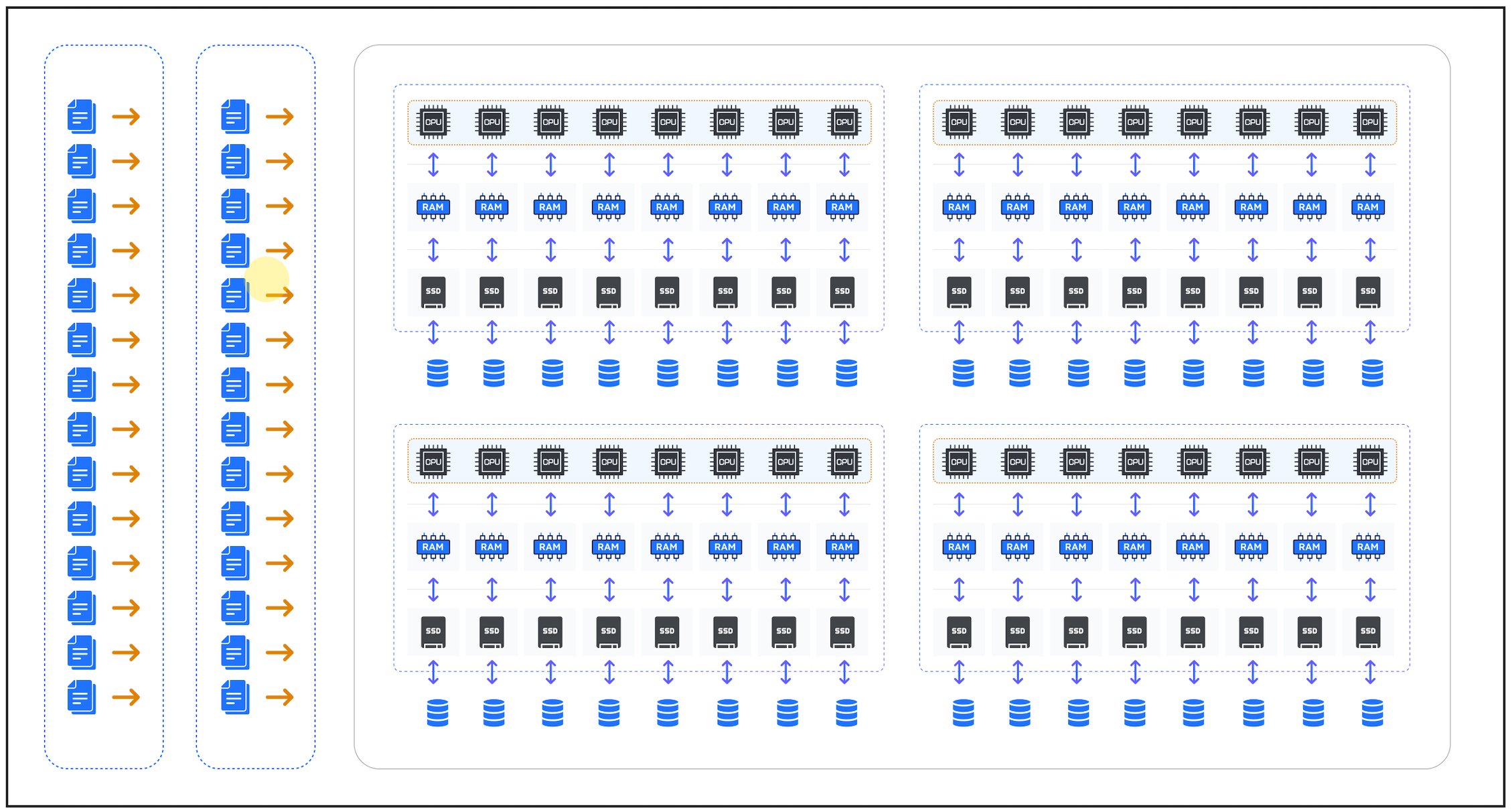
If you deliver hundreds of files, each file will be loaded in parallel on a separate CPU core with massive load performance. As a MEDIUM size warehouse has four servers, each with eight CPU cores, you can load up to 32 files in parallel, effectively improving load performance by 3,200%.

Be aware, however, it’s best practice to ensure data files are sized between 100-250MB, which means you’ll need a huge volume of data to justify splitting files. It’s, therefore, good practice to use just two warehouses to load all data into Snowflake. One XSMALL warehouse for single files (data loads of up to 250MB compressed), and another MEDIUM or larger warehouse for huge data loads split into file chunks of up to 250MB.

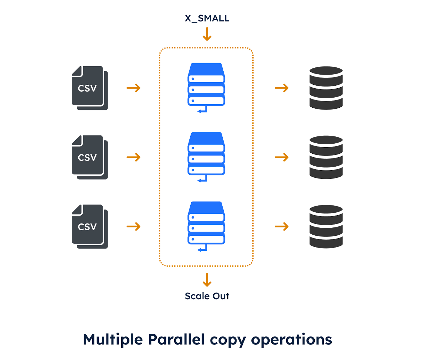
Remember, an XSMALL warehouse can load just eight files in parallel; during very busy times, you may be loading more than eight files in parallel. It’s, therefore, also a best practice to configure data-loading warehouses to use the Snowflake scale-out feature. The SQL statement below illustrates how:

create warehouse load_vwh with
   Warehouse_size = XSMALL
   min_cluster_count = 1
   max_cluster_count = 8
   auto_suspend = 30;

The diagram below illustrates how the solution works. It shows how multiple parallel COPY operations are executed on a single XSMALL warehouse. As the number of operations reaches eight parallel loads, Snowflake automatically adds additional servers to cope with the additional workload.

Conclusion

In conclusion, Snowflake deploys a revolutionary hardware and software architecture to maximize query performance, supporting scaling up (to a larger warehouse) and out (for more concurrent queries). Using the simple query performance strategies outlined in this article can greatly impact overall query performance, often for very little effort.

---

DataPilot from Altimate.ai can significantly improve Data Engineering productivity by not only finding the longest-running, most expensive queries but also narrowing them down to the specific lines of code to fix, providing AI-driven insights and detailed recommendations. If you, too, have a huge performance tuning backlog and are struggling to improve Snowflake operating costs or tuning query performance, why not get in touch?

Click on the image below to book a demo.